1 Introduction

In this section we want to compute how the light emitted by a linear light source is scattered by the atmosphere towards the camera (with a single scattering event, since we only deal with direct lighting here). For a small atmosphere segment on the path between the camera and a surface, this is given by a 1D integral over the infinitesimal elements of the light source. However, all the other segments along the path between the camera and a surface contribute in a similar way to the light received by the camera. We must therefore perform a second integration, along this path. The result is a double integral, which cannot be computed analytically. We could evaluate this double integral numerically at render time, but this would be way too costly for real-time rendering, and could also lead to discretization artifacts. Instead, we show here that, with some "reasonable" approximations (i.e., approximations yielding almost no perceptually visible differences in the final images), one of the integral can be precomputed in a 3D texture (but not the other, which must be evaluated numerically at runtime).

2 Model

Consider a linear light centered at $\bs$, of normal $\bn_s$, of width $w$ and length $2l$ and emitting a radiance $L_0$ in all directions of the upper $\bn_s$ hemisphere. We want to compute the light emitted by this source which is scattered by the atmosphere towards the camera $\bc$, along a view-ray from $\bc$ to a surface element $\bp$ (see Fig. 1).

Figure 1: Atmospheric scattering with a linear light source.

For a small segment centered at $\bq$ along the path from $\bc$ to $\bp$, the light which is scattered from a light source element centered at $\bs(x)$ towards the camera is the product of several terms:

the radiance $L_0$ times the solid angle of the light source element as seen from $\bq$, equal to $w\diff x\,\bn_s\cdot(\bq-\bs(x))/\Vert\bq-\bs(x)\Vert^3$
the atmospheric transmittance $\mathfrak{t}(\bs(x),\bq)$ between $\bs(x)$ and $\bq$,
a visibility term $V(\bs(x),\bq)$ indicating if $\bq$ is visible from $\bs(x)$,
the scattering coefficient $k_s(\bq)$ at $\bq$,
the scattering phase function $P$ depending on the angle between the $\bs(x)$-$\bq$ and $\bq$-$\bc$ segments,
the atmospheric transmittance $\mathfrak{t}(\bc,\bq)$ between $\bc$ and $\bq$.

Finally this product must be integrated over the light source elements $\bs(x)$ and over the path segments $\bq$. The resulting equation is \begin{equation} L_{LVE}(\bc,\bp)=\int_\bc^\bp\mathfrak{t}(\bc,\bq)k_s(\bq)\int_{-l}^{+l}P\left(\bs(x)-\bq,\bq-\bc\right)\frac{L_0w\,\bn_s\cdot(\bq-\bs(x))}{\Vert\bq-\bs(x)\Vert^3}\mathfrak{t}(\bs(x),\bq)V(\bs(x),\bq) \diff x \diff \bq\label{eq:exact} \end{equation}

Even with the analytic approximation for $\mathfrak{t}$ given in the Direct paths section, this double integral is too complicated to have an analytic solution. It also depends on too many parameters to be precomputed for all possible values. And computing this 2D integral numerically at each pixel at render time would be way too costly. Our solution to this problem is to make some approximations allowing us to precompute one of the integrals in a 3D texture. We are then left with a simpler 1D integral that we evaluate numerically at render time.

Approximations

Our main approximation is to replace $P$ with the isotropic phase function, equal to the $1/4\pi$ constant. For Rayleigh scattering this is justified by the fact that the Rayleigh phase function $3\pi(1+\mu^2)/16$ is not very directional, and by the fact that directional effects are averaged by the integral over the light source elements (see also the comparisons with "ground truth" images below). Note however that this is less justified for Mie scattering, which has a strong forward scattering component. This approximation yields \begin{align} L_{LVE}(\bc,\bp)&\approx\int_\bc^\bp \mathfrak{t}(\bc,\bq) J_{LV}(\bq) \diff \bq\label{eq:outer}\\ J_{LV}(\bq)&=\frac{L_0wk_s(\bq)}{4\pi}\int_{-l}^{+l}\frac{\bn_s\cdot(\bq-\bs(x))\mathfrak{t}(\bs(x),\bq)V(\bs(x),\bq)}{\Vert\bq-\bs(x)\Vert^3} \diff x\label{eq:inner} \end{align} where $J_{LV}(\bq)$ (in $W.m^{-3}$) can be seen as a volumetric light source, emitting light in all directions from all points. Since the light sources are at fixed positions, this source term can be precomputed and stored in a 3D texture (which can also include the contributions from the 6 linear light sources at once), which leaves "only" Eq. \eqref{eq:outer} to evaluate at runtime, using numerical integration.

3 Implementation

In order to store the precomputed source term $J_{LV}$ for all points inside Rama (more or less a cylinder) in a 3D texture (a cube), we must first define a mapping from this cylinder to a cube. If we include the 6 linear light sources in the same texture, the source term $J_{LV}(\bq)$ is symmetric under $120$ degrees rotations around the Rama axis. $J_{LV}(\bq)$ is also symmetric around the planes passing through the light sources and the Rama axis. Thus, we can precompute and store only $60$ degrees, and get the other values by using the symmetry and periodicity. Finally, in order to get better precision near the light sources (where the light intensity is larger), it is desirable to have more texture samples in these regions, compared to the others. This can be achieved with a non linear mapping between the cylindrical coordinates and the texture coordinates. After some experimentations, we chose the mapping defined by the following functions:

float xWarp(float x) {
  const float a = 0.2;
  const float A = 2.0;
  const vec4 B = vec4(
      (5.0 - A) / (5.0 - a),
      A / a,
      (16.0 - 5.0 - 2.0 * A) / (16.0 - 5.0 - 2.0 * a),
      A / a);
  const vec4 C = vec4(
     0.0,
     5.0 * (1.0 - A / a),
     5.0 + A - (5.0 + a) * B.z,
     16.0 * (1.0 - A / a));
  const float Bp = (24.0 - 16.0 - A) / (24.0 - 16.0 - a);
  const float Cp = 24.0 * (A - a) / (24.0 - 16.0 - a);
  float v = x * (x > 0.0 ? 1.0 : -16.0 / 16.5);
  vec4 y = v * B + C;
  float yp = v * Bp + Cp;
  return sign(x) * clamp(y.w, clamp(y.y, y.x, y.z), yp);
}

// Return the light which is scattered at x, supposed
// to be equal in all directions. x must be given in
// Rama coordinates (using kilometers units).
vec3 inscatterSource(vec3 x) {
  const vec3 RES = vec3(48.0, 32.0, 32.0) + vec3(1.0);
  vec3 u;
  u.x = (xWarp(x.x) + 24.0) / 48.0;
  u.y = 1.0 - length(x.yz) / (7.75 + clamp(x.x, -0.25, 0.25));
  u.z = atan(x.z, x.y) / (PI / 3.0);
  u.z = abs(u.z - 2.0 * floor(u.z * 0.5 + 0.5));
  u.yz = sqrt(u.yz);
  u = 0.5 / RES + u * (1.0 - 1.0 / RES);
  return texture3D(scatteringSampler, u).rgb;
}

where scatteringSampler is the precomputed 3D texture (of size $49\times 33\times 33$ pixels) containing $J$. We can then use the inscatterSource function to evalue Eq. \eqref{eq:outer} numerically:

// Return the light which is scattered towards p along the
// segment from p to p+d. p and d must be in Rama coordinates
// (using kilometers units).
vec3 atmosphericScattering(vec3 p, vec3 d) {
  const float SAMPLES = 30.0;
  vec3 result = vec3(0.0);
  for (float i = 0.0; i < SAMPLES; ++i) {
    vec3 x = p + (i + 0.5) / SAMPLES * d;
    result += transmittance(p, x) * inscatterSource(x);
  }
  return result / SAMPLES * length(d);
}

4 Results

The figure below compares the "ground truth" result obtained with a numerical integration of Eq. \eqref{eq:exact} (using $30\times 30$ samples per light source, which would require $5400$ samples per pixel for 6 light sources) and the results obtained with our approximation (using $30$ samples per pixel at render time, and $50$ samples per light source during precomputation).

Figure 2: Direct lighting of the atmosphere, for a single light source, using a precomputed 3D texture and $30$ samples per pixel.

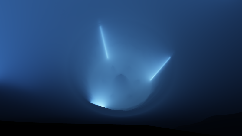
The result for the 6 light sources, using the same exposure, is the following:

Figure 3: Direct lighting of the atmosphere using a precomputed 3D texture and $30$ samples per pixel.