
Coupled Lighting and Temperature Profiles
|
Rama
physics Coupled Lighting and Temperature Profiles |
The goal of this section is to compute the lighting and temperature profiles at the surface and in the atmosphere of Rama, while taking the retroactions between the two into account, in the non axisymetric case. Indeed, until now, we computed the lighting and temperature profiles at the surface without atmosphere, and computed the atmosphere temperature and pressure by assuming that the surface lighting and temperature were uniform, i.e. axisymetric. The results are an almost uniform surface temperature, and a uniform atmosphere temperature. However, taking the retroactions between the surface and the atmosphere into account could invalidate these results. The goal of this section is to know whether this is the case or not.
The retroactions between the surface and the atmosphere are quite complex. For instance, temperature variations at the surface lead via radiative transfer to temperature variations in the atmosphere, which, via the ideal gas law, lead to pressure and/or density variations and, possibly, to the creation of winds inside the atmosphere. The pressure and density variations, in turn, lead to variations of the absorption and scattering coefficients, i.e. to changes in the variations of the lighting in the short wave range at the surface and in the atmosphere. These, in turn, lead to temperature variations.
To simplify computations, we assume here that the atmosphere is at rest and that the final temperature variations at the surface and in the atmosphere will be small (winds are studied in the next section). This allows us to suppose that the density profile of the atmosphere is the one computed in the previous section for the average surface temperature (indeed, we showed that this profile is almost independent of small temperature variations). This is of course an approximation, as it will not be possible to satisfy simultaneously the ideal gas law and the hydrostatic equilibrium equation in the end result. But it allows us to suppose the density and thus the absorption and scattering coefficients as given (by the equations in the previous section), instead of being functions of the unknowns of the problem.
Note that the above hypothesis simplifies computations, but we will then need to check if the results obtained with it are consistent or not. If we don't find small variations in the end, then the hypothesis is invalid, and we will need to take the full surface-atmosphere retroactions into account.
We note $E(\theta)$ the irradiance received at the surface in the short wave range, and $L(\theta)$ the radiance emitted at the surface in this same range. We also note $L(\bp,\bw)$ or $L(r,\theta,\bw)$ the radiance traveling at the point $\bp$ of cylindrical coordinates $(r,\theta)$ in direction $\bw$ in the atmosphere, in the short wave range. The irradiance $E$ is given, from the definition of the irradiance, by \begin{equation} E(\theta)=\int_{2\pi}L(r_s,\theta,\bw)\,\bn(\theta)\cdot\bw\,\diff\bw\label{eq:E} \end{equation} where the integral is taken over all the directions in the free hemisphere above $\bp$. The emitted radiance $L$ is given by the same equation as before: \begin{equation} L(\theta)=\frac{\alpha}{\pi}E(\theta)+L_0(\theta)\label{eq:L} \end{equation} with $L_0(\theta)=S/\pi r_s \Delta\theta$ for $-\Delta\theta/2<\theta<\Delta\theta/2$, and 0 otherwise (for a single light source). Finally, since there is no atmospheric absorption in the short wave range (at least this is the hypothesis we made from the beginning), and no thermal emission, the radiative transfer equation becomes: \begin{equation} \bw\cdot\nabla L(\bp,\bw)=-k_s(\bp)L(\bp,\bw)+k_s(\bp)\int_{4\pi}P(\bw,\bw')L(\bp,\bw')\diff\bw'\label{eq:transfer} \end{equation} which always satisfies the radiative equilibrium equation $\nabla\cdot\mathbf{L}=0$ (see the previous section). These 3 equations, with the fact that $L(r_s,\theta,\bw)=L(\theta)$ for $\bw$ in towards the inside (which comes from our definitions), are the equations we must solve in order to find the coupled surface-atmosphere lighting profiles.
The formal solution to Eq. \eqref{eq:transfer} is given by \begin{equation} L(\bp,\bw)=L(\theta_{\bq})\mathfrak{t}_s(\bp,\bq)+\int_{\bp}^{\bq}k_s(\bx)\left(\int_{4\pi}P(\bw,\bw')L(\bx,\bw')\diff\bw'\right)\mathfrak{t}_s(\bp,\bx)\diff x \end{equation} where $\bq$ is the intersection point of the ray originating from $\bp$ and of direction $-\bw$ with the surface, and where $\mathfrak{t}_s$ is the transmittance due the scattering only (since there is no absorption in the short wave range). This equation can be interpreted as the radiance $L(\theta_{\bq})$ emitted at $\bq$, attenuated between $\bq$ and $\bp$ by the out-scattering, plus the integral over all the points $\bx$ along the path from $\bp$ to $\bq$ of the in-scattered radiance at $\bx$, attenuated between $\bq$ and $\bp$ by the out-scattering. Note that this is only a formal solution, since $L$ appears on both sides of the equation.
Substituting Eqs. \eqref{eq:E} and \eqref{eq:L} in this formal solution, we get \begin{equation} \begin{split} L(\bp,\bw)=&L_0(\theta_{\bq})\mathfrak{t}_s(\bp,\bq)+\frac{\alpha}{\pi}\left(\int_{2\pi}L(r_s,\theta_{\bq},\bw)\,\bn(\theta_{\bq})\cdot\bw\,\diff\bw\right)\mathfrak{t}_s(\bp,\bq)\\ &+\int_{\bp}^{\bq}k_s(\bx)\left(\int_{4\pi}P(\bw,\bw')L(\bx,\bw')\diff\bw'\right)\mathfrak{t}_s(\bp,\bx)\diff x \end{split}\label{eq:full} \end{equation} which is of the form $L=I_0+\mathcal{F}[L]$. The solution is therefore $L=I_0+\mathcal{F}[I_0]+\mathcal{F}[\mathcal{F}[I_0]]+\ldots$ This solution can't be computed analytically, but is also complex to compute numerically. Indeed, $L$ has 4 parameters ($r$, $\theta$, and 2 angles for $\bw$), and must therefore be stored in 4 dimensional arrays. Also a large resolution must be used for the directions, at least for the first terms, due to the small angular size $\Delta\theta$ of the linear light sources. We therefore use another strategy to solve this, explained below.
In order to simplify the resolution of Eq. \eqref{eq:full} we make here another hypothesis, namely that: \begin{equation} \int_{4\pi}P(\bw,\bw')L(\bx,\bw')\diff\bw'\approx\frac{1}{4\pi}\int_{4\pi}L(\bx,\bw)\diff\bw=J(\bx) \end{equation} We justify this by the fact that the phase function $P(\bw,\bw')$ for the Rayleigh scattering by the air molecules is not strongly anisotropic. Likewise, the 3 linear light sources plus the lighting from the surface (coming from all directions) give a radiance field which is not strongly anisotropic either. The average of the product of the two can therefore be assumed to be approximatively isotropic.
The Mie scattering from the aerosols is in general strongly anisotropic. Our hypothesis is thus equivalent to say that there are no aerosols (e.g. pollution) in Rama.
Using this approximation, we can rewrite Eq. \eqref{eq:full} as \begin{equation} L=\cT[\pi L_0]+\alpha\cT[\cE[L]]+\cS[\cJ[L]]\label{eq:func} \end{equation} where the linear operators $\cT$, $\cE$, $\cJ$ and $\cS$ are defined by \begin{align} \cT[E](\bp,\bw)&\eqdef\frac{1}{\pi}E(\theta_{\bq})\mathfrak{t}_s(\bp,\bq)\\ \cE[L](\theta)&\eqdef\int_{2\pi}L(r_s,\theta,\bw)\,\bn(\theta)\cdot\bw\,\diff\bw\\ \cJ[L](\bp)&\eqdef\frac{1}{4\pi}\int_{4\pi}L(\bp,\bw)\diff\bw\\ \cS[J](\bp,\bw)&\eqdef\int_{\bp}^{\bq}k_s(\bx)J(\bx)\mathfrak{t}_s(\bp,\bx)\diff x \end{align} We also have $E(\theta)=\cE[L](\theta)$ and $J(\bp)=\cJ[L](\bp)$. Substituting Eq. \eqref{eq:func} into this, we get \begin{align} E&=\cE[\cT[\pi L_0]]+\alpha\cE[\cT[E]]+\cE[\cS[J]]]\\ J&=\cJ[\cT[\pi L_0]]+\alpha\cJ[\cT[E]]+\cJ[\cS[J]]] \end{align} which can be rewritten as \begin{align} E&=E_0+\alpha\cF_1[E]+\cF_2[J]\label{eq:Er}\\ J&=J_0+\alpha\cF_3[E]+\cF_4[J]\label{eq:Jr} \end{align} by using the following definitions: \begin{equation} E_0\eqdef\cF_1[\pi L_0],\, J_0\eqdef\cF_3[\pi L_0],\, \cF_1\eqdef\cE\circ\cT,\, \cF_2\eqdef\cE\circ\cS,\, \cF_3\eqdef\cJ\circ\cT,\, \cF_4\eqdef\cJ\circ\cS \end{equation}
The solution of this system of two equations is given by two infinite series \begin{align} E&=E_0+E_1+E_2+\ldots\\ J&=J_0+J_1+J_2+\ldots \end{align} where \begin{align} E_{n+1}&\eqdef\alpha\cF_1[E_n]+\cF_2[J_n]\label{eq:En1}\\ J_{n+1}&\eqdef\alpha\cF_3[E_n]+\cF_4[J_n]\label{eq:Jn1} \end{align} as can be verified as follows: \begin{align*} E&=\sum_{i=0}^\infty E_i=E_0+\sum_{i=0}^\infty E_{i+1}=E_0+\sum_{i=0}^\infty \alpha\cF_1[E_i]+\cF_2[J_i]\\ &=E_0+\alpha\cF_1[\sum_{i=0}^\infty E_i]+\cF_2[\sum_{i=0}^\infty J_i]=E_0+\alpha\cF_1[E]+\cF_2[J] \end{align*} which is Eq. \eqref{eq:Er} - a similar derivation can be made for Eq. \eqref{eq:Jr}. Note that these series have a simple physical interpretation: the $E_i$ term corresponds to the radiance received on the ground after exactly $i$ bounces on the ground or in the atmosphere, and the $J_i$ term corresponds to the average radiance received in the atmosphere after exactly $i$ bounces on the ground or in the atmosphere.
Note also that $E$ and $J$ are functions of 1 and 2 parameters respectively. They are therefore much easier to store with a high resolution than the 4 parameters function $L$. Also $E_0$ and $J_0$ don't need a very high resolution to be accurately represented numerically, unlike $L_0$. All this make the numeric computation of $E$ and $J$ much easier to do than the direct computation of $L$. And once $E$ and $J$ are known, $L$ can be found directly with $L=\cT[\pi L_0+\alpha E]+\cS[J]$.
The operators $\cF_1$, $\cF_2$, $\cF_3$ and $\cF_4$ correspond respectively to the surface irradiance, volume irradiance, average surface radiance, and average volume radiance computed in the Appendix. Using their value, we can rewrite Eqs. \eqref{eq:En1} and \eqref{eq:Jn1} in an expanded form: \begin{align*} E_{n+1}(\theta)=&\frac{\alpha}{4}\int_{2\pi}E_n(\theta')f_2(\mathfrak{t}_s(r_s,\theta,r_s,\theta'))\vert\sin\frac{\theta'-\theta}{2}\vert \diff\theta'\\ &+2\int_{2\pi}\int_0^{r_s}k_s(r)J_n(r,\theta')f_1(\mathfrak{t}_s(r_s,\theta,r,\theta'))\frac{r(r_s-r\cos(\theta'-\theta))}{r_s^2+r^2-2rr_s\cos(\theta'-\theta)}\diff r\diff\theta'\\ J_{n+1}(r,\theta)=&\frac{\alpha}{2\pi^2}\int_{2\pi}E_n(\theta')f_1(\mathfrak{t}_s(r,\theta,r_s,\theta'))\frac{r_s(r_s-r\cos(\theta'-\theta))}{r_s^2+r^2-2rr_s\cos(\theta'-\theta)}\diff\theta'\\ &+\frac{1}{4}\int_{2\pi}\int_0^{r_s}k_s(r')J_n(r',\theta')f_0(\mathfrak{t}_s(r,\theta,r',\theta'))\frac{r'}{\sqrt{r^2+r'^2-2r'r\cos(\theta'-\theta)}}\diff r'\diff\theta' \end{align*} where $f_n(x)\eqdef\int_0^{\pi/2}x^{1/\cos\phi}\cos^n\phi\diff\phi/\int_0^{\pi/2}\cos^n\phi\diff\phi$ and $\mathfrak{t}_s$ is the transmittance of the atmosphere due to the out-scattering only. Note that if $k_s=0$ then $\mathfrak{t}_s=1$ and we get $E_{n+1}(\theta)=\frac{\alpha}{4}\int_{2\pi}E_n(\theta')\vert\sin\frac{\theta-\theta'}{2}\vert \diff\theta'$, which is what we got for the lighting profile without atmosphere.
We can also compute $E_0$ and $J_0$. If we approximate the light source width $\Delta\theta$ with a Dirac we get (for a single light source): \begin{align*} E_0(\theta)&\approx\frac{S}{4r_s}f_2(\mathfrak{t}_s(r_s,\theta,r_s,0))\vert\sin\frac{\theta}{2}\vert\\ J_0(r,\theta)&\approx\frac{S}{2\pi^2 r_s}f_1(\mathfrak{t}_s(r,\theta,r_s,0))\frac{r_s(r_s-r\cos(\theta))}{r_s^2+r^2-2rr_s\cos(\theta)} \end{align*} This is fine for $E_0$, but $J_0$'s approximation diverges towards $+\infty$ at the light source ($r=r_s$ and $\theta=0$). To avoid this divergence we use a better approximation: we still approximate the $f_1$ term with a constant in the integral, but we integrate the other term (i.e. the fraction) analytically, without approximation. This gives: \begin{equation*} J_0(r,\theta)\approx\frac{S}{2\pi^2 r_s\Delta\theta}f_1(\mathfrak{t}_s(r,\theta,r_s,0))\big(F(r, -\theta+\frac{\Delta\theta}{2})-F(r, -\theta-\frac{\Delta\theta}{2})\big) \end{equation*} where \begin{equation*} F(r, \theta)\eqdef\tan^{-1}\left(\frac{r-r_s}{r+r_s}\cot\frac{\theta}{2}\right)+\frac{\theta}{2}+\pi\left\lfloor\frac{\theta}{2\pi}\right\rfloor \end{equation*} is the indefinite integral of the fraction term. With this better approximation $J_0$ does not diverge, and its maximum value, reached at $r=r_s$ and $\theta=0$ is \begin{equation*} J_0^{max}=\frac{S(\Delta\theta+\pi)}{2\pi^2 r_s\Delta\theta}\approx\frac{S}{2\pi r_s\Delta\theta} \end{equation*}
The above equations can't be solved analytically. We therefore use numerical integration instead. Our method for doing this is detailed in the Appendix. The results are the following.
The irradiance $E(\theta)$, shown in Fig. 1, is similar to the result found without atmosphere, except that we now have 3 small spikes, located at the light sources. Also, if we except these spikes, the lighting variations are smaller than without atmosphere (5.5% instead of 13% - but 28% with the spikes). These two differences are due to the scattering of light in the atmosphere:
Note also that the average value is the same with or without atmosphere, as was shown in the beginning.

The average radiance $J(r,\theta)$ in the atmosphere, shown in Fig. 2, has much larger variations. Indeed, $J$ varies between 0.55 and 5100 times its average value $J^{avg}=S/2\pi^2 r_s(1-\alpha)$ - we use $\Delta\theta=\pi/18000=0.01°$, yielding $J^{max}/J^{avg}\approx$ $J_0^{max}/J^{avg}=$ $18000(1-\alpha)/3=5100$). However, as can be seen in Fig. 2, the really large values of $J$ are restricted to a small area near the light sources: values larger than 5 times the average are limited to a cylinder of $\approx 500\,m$ diameter above each light source.

We note $\bar{E}^{\downarrow}(\theta)$ and $\bar{E}^{\uparrow}(\theta)$ the irradiance respectively received and emitted in the long wave range, and $\bar{L}(\bp,\bw)$ the radiance traveling at $\bp$ in direction $\bw$ in the long wave range inside the atmosphere. The same equation as before holds for the net flux at the ground level: \begin{equation} E(\theta)+\bar{E}^{\downarrow}(\theta)=\alpha E(\theta)+(1+\frac{1}{\Delta})\bar{E}^{\uparrow}(\theta) \end{equation} The radiance $\bar{L}$ satisfies the radiative transfer equation. In the long wave range there is no scattering (Rayleigh scattering is inversely proportional to $\lambda^4$ and is thus very small in the long wave range). This equation is thus: \begin{equation} \bw\cdot\nabla \bar{L}(\bp,\bw)=-k_e(\bp)\bar{L}(\bp,\bw)+k_e(\bp) \frac{\sigma T^4(\bp)}{\pi} \end{equation} whose formal solution is \begin{equation} \bar{L}(\bp,\bw)=\frac{1}{\pi}\bar{E}^{\uparrow}(\theta_{\bq})\mathfrak{t}_e(\bp,\bq)+\int_{\bp}^{\bq}k_e(\bx)\frac{\sigma T^4(\bx)}{\pi}\mathfrak{t}_e(\bp,\bx)\diff x \end{equation} This solution does not automatically satisfy the radiative equilibrium equation $\nabla\cdot\mathbf{L}=0$, which must therefore be added (see the previous section): \begin{equation} \frac{1}{4\pi}\int_{4\pi}\bar{L}(\bp,\bw)\diff\bw=\frac{\sigma T^4(\bp)}{\pi} \end{equation} Finally, the last equation needed to compute the temperature profile is the definition of the received irradiance: \begin{equation} \bar{E}^{\downarrow}(\theta)=\int_{2\pi}\bar{L}(r_s,\theta,\bw)\,\bn(\theta)\cdot\bw\,\diff\bw \end{equation} where the integral is taken over all the directions in the free hemisphere above $\bp$.
Using the same operators $\cT$, $\cE$, $\cJ$ and $\cS$ as above, with $k_s$ and $\mathfrak{t}_s$ replaced with $k_e$ and $\mathfrak{t}_e$, these equations can be rewritten as: \begin{align} \bar{E}^{\uparrow}&=(1-\alpha)\bar{\alpha} E+\bar{\alpha} \bar{E}^{\downarrow}\\ \bar{L}&=\cT[\bar{E}^{\uparrow}]+\cS[\cJ[\bar{L}]]\\ \bar{E}^{\downarrow}&=\cE[\bar{L}]\\ \bar{J}\eqdef\cJ[\bar{L}]&=\sigma T^4/\pi \end{align} from which we get \begin{align} \bar{L}&=\cT[(1-\alpha)\bar{\alpha} E]+\bar{\alpha}\cT[\bar{E}^{\downarrow}]+\cS[\bar{J}]\\ \bar{E}^{\downarrow}&=\cF_1[(1-\alpha)\bar{\alpha} E]+\bar{\alpha}\cF_1[\bar{E}^{\downarrow}]+\cF_2[\bar{J}]\\ \bar{J}&=\cF_3[(1-\alpha)\bar{\alpha} E]+\bar{\alpha}\cF_3[\bar{E}^{\downarrow}]+\cF_4[\bar{J}] \end{align} Note that these equations have exactly the same form as Eqs. \eqref{eq:func}, \eqref{eq:Er} and \eqref{eq:Jr} and can therefore be solved numerically in exactly the same way.
Again, the temperature profiles equations can't be solved analytically. We therefore use numerical integration instead and our method for doing this is detailed in the Appendix. The results are the following.
The emitted irradiance $\bar{E}^{\uparrow}(\theta)$ in the long wave range, shown in Fig. 3, is similar to the result found without atmosphere, except that we now have 3 small spikes, located at the light sources. Also, without the spikes, the irradiance variations are smaller than without atmosphere: the maximum irradiance is 2.6% larger than the minimum irradiance, instead of 5.4% without atmosphere, for the "incandescent" scenario $\Delta=1.3$ (resp. 1.6% instead of 3% for the "energy saving" scenario $\Delta=2.9$). These two differences can be easily explained:
Note also that the average value is the same with or without atmosphere, as was shown in the beginning.

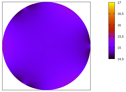
By converting the irradiance to temperatures with the relation $E=\sigma T^4$, we get the variations shown in Fig. 4: the temperature delta is less than 2°C in both scenarios, except in very small regions near the light sources (about 0.5°, i.e. about 70 m on each side of each light source) where it reaches about 7°C in the incandescent scenario (resp. about 5°C in the energy saving scenario).

Similarly, we also get very small variations for the average radiance in the long wave range in the atmosphere, $\bar{J}(r,\theta)$. These variations, converted to temperatures, are shown in Fig. 5 and Fig. 6 for the incandescent and energy saving scenarios, respectively. Except for a very small region near each light source, which is too small to be seen in the figures, the temperature delta is about 2°C in the incandescent scenario, and about 1° in the energy saving scenario. And even with the regions near the light sources taken into account, the temperature delta is less than 5°C (resp. 3°C).

However, it is important to note that we get these very small atmospheric temperature variations - especially when compared to the very large variations in the short wave range - only because the atmosphere does not absorb any radiation in the short wave range (at least this is what we assumed from the beginning). For comparison, we can compute the temperature of a small black body object in the atmosphere: this object would absorb $J+\bar{J}$ watts per square meter in average. Converted to temperatures, this gives the profiles shown in Fig. 7 and Fig. 8 for the incandescent and energy saving scenarios, respectively.


The temperatures vary between 47°C (on the ground at mid distance between two light sources) and 2100°C (directly above a light source) in the incandescent scenario, and between 30°C and 1670°C in the energy saving scenario. We can also see from the two figures that a small object in the atmosphere would have much a more comfortable temperature in the energy saving scenario than in the incandescent scenario.
When the atmosphere is taken into account, as well as some retroactions between the atmosphere and the ground, the temperature variations we obtain are very small. In fact, they are even smaller than in the no atmosphere case, if we except small spikes near the light sources (and they remain small even if the spikes are taken into account). This can be explained by the fact that the scattering of light and the absorption and re-emission of thermal infrared radiations in the atmosphere tend to average the radiations over all directions, and thus over all locations as well.
Finally, note that these results are consistent with the small variations hypothesis we made at the beginning (which allowed us to suppose that the atmosphere density profile is approximatively the same as in the axisymmetric case), which thus validates this hypothesis and our results.